Chapter 2. Producers and supply
1 Production function
A production function describes how inputs (factors of production such as labor, capital and land, etc.) can be transformed into outputs. We denote the production function by \(f:\mathbb{R}^n\to\mathbb{R}_+\), where \(n\) is the number of inputs. In the case of two inputs, capital (\(K\)) and labor (\(L\)): \[ q = f(K, L), \] where \(q\) is the amount of output.
Example 1
Cobb-Douglas production function: \(q = AK^{\alpha}L^{\beta}\), where \(A>0\) and \(\alpha, \beta \in (0,1)\)
Leontief production function: \(q = A\min\{aK, bL\}\), where \(A, a, b>0.\) This production function captures the idea that inputs must be used in fixed proportion
Linear production function: \(q = aK + bL\) where \(a, b > 0.\) Here inputs are perfectly substitutable (e.g., robots vs human workers in the future)
Quasilinear production function: \(q = AK^a + bL\) where \(A, a, b>0.\) This production function could be used to capture different returns to scales of different inputs. For example scaling is quite straightforward for labor or raw materials but might be complex for capital and land.
The Cobb-Douglas, linear and fixed-proportion production functions are all special cases of the CES production function: \[ q = \left(aL^{\frac{s-1}{s}} + bK^{\frac{s-1}{s}}\right)^{\frac{s}{s-1}}, \tag{1}\]
where \(s\) is the EoS. Special cases:
- As \(s\to \infty\): CES \(\to\) linear production function
- As \(s \to 0\): CES \(\to\) fixed-proportion production function
- As \(s \to 1\): CES \(\to\) the Cobb-Douglas production function
Why is it called CES? Let \(q(L, K)\) be a twice differentiable production function of two inputs. The elasticity of substitution between the two factors measures the percentage in the ratio of the inputs in response to a percentage change in the MRTS. Mathematically:
\[ s = \frac{d\ln \left(\frac{K}{L}\right)}{d \ln MRTS_{K,L}}, \tag{2}\]
where \(MRTS_{K,L} = MP_L/MP_K\) is the marginal of technical substitution of capital for labor. It measures the rate at which the firm is willing to replace labor with capital while keeping output constant. The EoS is a measure of how easily the firm can substitute one input for another.
2 Average and marginal products
2.1 Average product and productivity
The average product is the total units of output produced per unit of input used
- The average product or productivity of labor, \(AP_L = q / L\)
- The average product or productivity of capital, \(AP_K = q / K\)
The higher is the average product, the higher is the productivity. Productivity typically depends on the production technology and the levels of input used.
Example 2 For each of the following production functions, compute the average product of labor (or labor productivity). Determine if increasing labor improves productivity.
- \(q = 100 \sqrt{L}\)
- \(q = 5 L^{1/2} + 3L - 6\)
2.2 Marginal product
The marginal product is the rate at which total output changes as the firm uses one additional unit of input
The marginal product of labor: \(MP_L = \frac{\Delta q}{\Delta L}\) when \(L\) is discrete (e.g. number of workers) and \(MP_L = \frac{\partial q}{\partial L}\) when \(L\) is continuous (e.g. working hours)
The marginal product of capital: \(MP_K = \frac{\Delta q}{\Delta K}\) when \(K\) is discrete and \(MP_K = \frac{\partial q}{\partial K}\) when \(K\) is continuous
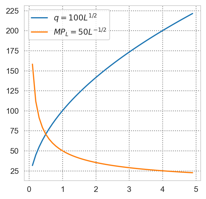
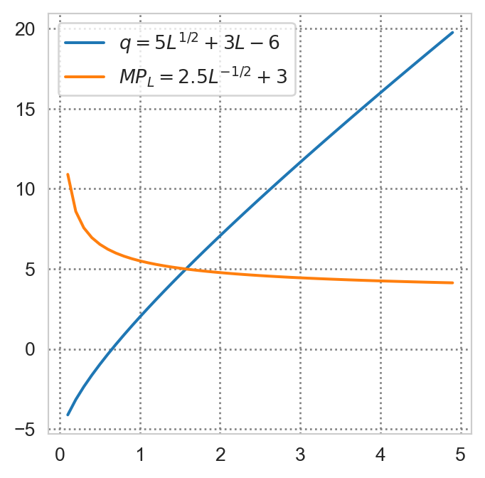
Example 3 Compute the marginal product of labor for the production functions in Example 2 and determine if it is increasing or decreasing in the amount of input used.
2.3 Decreasing marginal products
Marginal products are typically decreasing in the amount of input used. This is known as the law of diminishing marginal products. This is because the other inputs are held fixed. For example, consider a firm that produces a certain good using labor and capital. If the firm hires more workers but does not increase the amount of capital, then each additional worker has less capital to work with, which reduces their productivity.
2.4 Relationship beteen average and marginal products
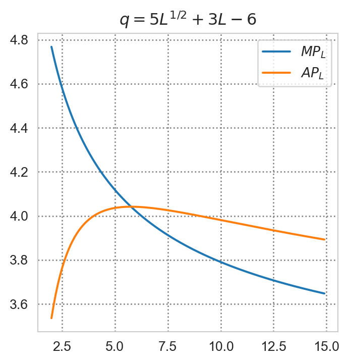
Figure 3 suggests that the AP curve crosses the MP curve at its maximum. In particular, as the AP is increasing when it is less than the MP and it is decreasing when it is greater than the MP. This makes sense intuitively since the MP being greater than the AP means the added worker is more productive than the average worker in the existing team, and vice versa.
Let us formalize this observation. Consider the case of continuous labor input and differentiable production function. Let \(\bar{q}(L) = q(L) / L\) be the average product. Differentiating with respect to \(L\) yields:
\[ \begin{aligned} \bar{q}'(L) &= \frac{q'(L)L - q(L)}{L^2}, \quad L > 0. \\ \bar{q}'(L) \geq 0 &\iff q'(L)L - q(L) \geq 0 \\ &\iff q'(L) \geq \frac{q(L)}{L} \\ &\iff q'(L) \geq \bar{q}(L). \end{aligned} \tag{3}\]
Thus the average product, \(\bar{q}\), is increasing when the marginal product \(q'\) is greater than the average product and is decreasing otherwise.
3 Isoquants
3.1 Definition
In the first chapter, we saw that indifference curves (also known as isoutility curves) are nothing but the level curves of the utility function that represents a consumer’s preference relation. In particular, each IC represents combinations of goods that give the consumer the same level of utility.
Isoquants are to firms is a similar (but not identical) concept: Each isoquant represents all combinations of inputs that yield the same level of output given the firm’s production technology, but the the levels assocated with the isoquants are cardinal: they represent actual outputs, not just fictive units that are only used for ranking alternatives. This implies that a monotone transformation of the production function does not yield the same isoquants, unlike in the case of indifference curves.
3.2 Example
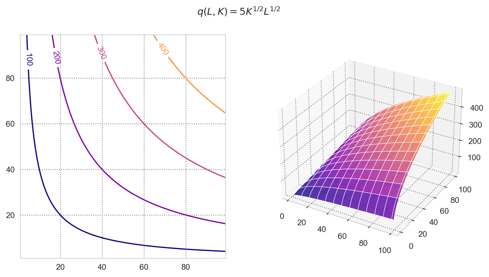
Consider the production function \(q(K, L) = 5K^{1/2} L^{1/2}\). We would like to find the the isoquant corresponding to \(m > 0\) units of output.
Observe that \(m > 0\) implies that both inputs are strictly positive. We have: \[ 5K^{1/2} L^{1/2} = m \\ \iff K = \frac{m^2}{25L}. \]
4 Marginal rate of technical substitution (MRTS)
4.1 Definition
The MRTS is the slope of the isoquant (in absolute value):
\[ \frac{-dK}{dL} = \frac{MP_L}{MP_K} \equiv MRTS_{K,L}. \tag{4}\]
It tells us how many units of capital the firm is willing to give up in order to hire one additional worker while keeping output constant. It is decreasing as the amount of labor increases, which is consistent with the law of diminishing marginal products (the additional worker is less productive than the previous one, so the firm is willing to give up less capital to hire them).
As in the case of MRS, we derive the MRTS by totally differentiating along an isoquant, where \(q(L, K) = m\) for some constant \(m>0\):
\[ \begin{aligned} df(L, K) &= 0 \\ \iff f_L dL + f_K dK &= 0 \\ \iff \frac{-dK}{dL} &= \frac{f_L}{f_K} \\ &= \frac{MP_L}{MP_K} \equiv MRTS_{K, L}. \end{aligned} \tag{5}\]
4.2 Properties
In the case of Cobb-Douglas production function above, the MRTS is decreasing as we move in the south-east direction along one isoquant:
- When capital is abundant, the firm is willing to give up many units of capital to hire an additional worker (the isoquant is steep). When capital is scarce, the firm is willing to give up only a few units of capital to hire an additional worker (the isoquant is flat).
How about the case of linear production function? And the case of fixed input proportions?
5 Homogeneity and returns to scale
Let \(\alpha > 0\) be the factor by which all inputs change (i.e., each input is multiplied by \(\alpha\)). Suppose \(f(\alpha K, \alpha L) = \alpha^k f(K, L)\) for some number \(k\)
- If \(k > 1\): the firm exhibits increasing returns to scale (IRS)
- If \(k = 1\): the firm exhibits constant returns to scale (CRS)
- If \(k < 1\): the firm exhibits decreasing returns to scale (DRS)
Note that the characterization holds regardless of whether \(\alpha\) is greater or smaller than one. If \(\alpha \in (0, 1)\) then increasing returns to scale means that as we reduce inputs by a factor of \(\alpha\), the firm’s output falls by more than \(\alpha\).
In practice, different activities within the same firm or industry may exhibit different returns to scale. In the automobile industry, for example, design is a nonrival input: a single platform can serve any number of vehicles, so scaling all inputs, including design, raises output more than proportionally (IRS). Assembly, by contrast, exhibits approximately CRS beyond a minimum efficient scale, since it expands by replicating plants and production lines. At the level of the whole firm, coordination and management costs may eventually generate DRS.
Example 4 Consider the Cobb-Douglas production function \(q = AK^a L^b\) where \(A, a, b\) are strictly positive constants. For which values of \(a, b\) does this function exhibit increasing, constant or decreasing returns to scale? What kind of returns to scale do linear and fixed-proportion production functions exhibit?
Answer
- Cobb-Douglass:
For some \(\alpha > 0\), we have: \[ \begin{aligned} f(\alpha L, \alpha K) &= A \alpha^{a+b} K^a L^b \\ &= \alpha^{a+b} f(L, K). \end{aligned} \tag{6}\]
Hence the nature of returns to scale depends on \(a+b\). In particular:
- IRS if \(a+b > 1\)
- DRS if \(a+b < 1\)
- CRS if \(a+b = 1\)
- Linear and fixed-proportion production functions both exhibit CRS
Exercise 1 Show that if a production function is homogeneous of degree \(k\), then the marginal products are homogeneous of degree \(k-1\).
6 Technological progress
A technical progress is a technical advance that allows firms to produce more with the same amount of inputs. In general a technical progress can be:
- Labor enhancing if MPL increases by more than MPK
- Capital enhancing if MPK increases by more than MPL
- Neutral if MPL and MPK increase by the same proportion
Hence to determine the nature of the tech progress, we need to compare the relative change of the productivity of labor and capital following the change in the production technology. The percentage change in the marginal product of each input can be expressed as: \[ \frac{MP'_i - MP_i}{MP_i} = \frac{MP'_i}{MP_i} - 1, \quad i\in\{K, L\}, \] where \(MP'_i\) denotes the marginal product of input \(i\) after the technological progress. Observe that: \[ \begin{aligned} \frac{MP'_L - MP_L}{MP_L} &\geq \frac{MP'_K - MP_K}{MP_K} \\ % \iff \frac{MP'_L}{MP_L} \geq \frac{MP'_K}{MP_K} \\ % \iff \frac{MP'_L}{MP'_K} \geq \frac{MP_L}{MP_K} \\ MRTS'_{K, L} &\geq MRTS_{K, L}. \end{aligned} \]
Hence the type of the technical progress can be determined by comparing the MRTSs. In particular, if \(MRTS'_{K, L} > MRTS_{K, L}\), then the technical progress is labor enhancing since each worker must be replaced by more capital, implying that labor has become more productive following the progress.
Example 5 Suppose the firm has production function \(f = A_1 L^a K^b\). After a technical progress, it has one of the following PFs.
- \(f = A_1 L^{a + \delta} K^b\) with \(\delta > 0\)
- \(f = A_1 L^a K^{b + \delta}\) with \(\delta > 0\)
- \(f = A_2 L^a K^b\) with \(A_2 > A_1\)
Let us determine the type of progress that the firm has undergone.
Labor-enhancing technological progress
Consider \(f = A_1 L^{a + \delta} K^b\) with \(\delta > 0\) The MRTS before tech progress: \[ MRTS_{L,K} = \frac{a}{b}\frac{K}{L}. \] After tech progress: \[ MRTS'_{L,K} = \frac{a+\delta}{b}\frac{K}{L}. \]
Since \(\delta > 0\), we have \(MRTS'_{L,K} > MRTS_{L,K}\), implying that this is a labor-enhancing (or labor-saving) tech progress. Graphically, on the \((K, L)\) plane, the isoquants become steeper
Capital-enhancing technological progress
Consider \(f = A_1 L^a K^{b + \delta}\) with \(\delta > 0\). The MRTS before tech progress: \[ MRTS_{L,K} = \frac{a}{b}\frac{K}{L}. \] After tech progress: \[ MRTS'_{L,K} = \frac{a}{b+\delta}\frac{K}{L}. \]
Since \(\delta > 0\), we have \(MRTS'_{L,K} < MRTS_{L,K}\), which is equivalent to \(MRTS'_{K,L} > MRTS_{K,L}\), implying that this is a capital-enhancing (capital-saving) tech progress. How do the isoquants change graphically?
Neutral technological progress
In the final example \(f = A_2 L^a K^b\) with \(A_2 > A_1\), the \(MRTS\) does not change after the progress, implying that this is a neutral one. Graphically the isoquants do not change.
7 Cost functions
7.1 Isocost lines
Definition 1 (Isocost) An isocost line is the set of input combinations that yield the same total cost (TC) for the firm. Mathematically, let \(w>0\) and \(r>0\) be the prices of labor and capital, respectively. Then the isocost consists of all \((w, r)\) pairs such that: \[ TC = wL + rK. \tag{7}\]
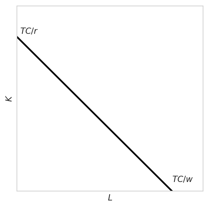
Observe that the slope of the isocost line is \(-w/r\), implying that as \(w\) rises, this line gets steeper.
7.2 Cost minimization problem (CMP)
The cost minimization problem entails finding a combination of inputs that minimizes the total cost of production for a given level of output.
Definition 2 (CMP) \[ \begin{aligned} &\min_{L,K} C = wL + rK \\ &\text{s.t. } f(L, K) \geq m, \end{aligned} \tag{8}\] where \(m\) is the target output level.
The idea is to identify the isocost line touching the isoquant that is as close to the origin as possible.
7.2.1 Necessary conditions
The Lagrangian of the CMP: \[ \mathcal{L}(\lambda, L, K) = - C(L, K) + \lambda (f(L,K) - m). \tag{9}\]
According to the KTT theorem, if \((L^*, K^*)\) is a solution to the CMP, then there exist \(\lambda^* \geq 0\) such that:
\[ \begin{aligned} &\mathcal{L}_L (L^*, K^*, \lambda^*) = 0, \: \mathcal{L}_K (L^*, K^*, \lambda^*) = 0, \\ % &\quad \quad \quad \text{ with equality for interior solutions }\\ &\lambda^* \geq 0, \: f(L^*, K^*) - m \geq 0, \: \lambda^*[f(L^*, K^*) - m] = 0. \end{aligned} \tag{10}\]
The FOCs yield: \[ \begin{aligned} \lambda^* f_L(L^*, K^*) &= w, \\ \lambda^* f_K(L^*, K^*) &= r. \end{aligned} \tag{11}\]
This implies: \[ \begin{aligned} \frac{MP_L}{MP_K} &= \frac{w}{r} \\ \frac{MP_L}{w} &= \frac{MP_K}{r}=\frac{1}{\lambda^*}. \end{aligned} \tag{12}\]
Note that \(\lambda^*\) here, the shadow price, represents the cost of increasing output by a unit: \[ \lambda^* = \frac{\partial C^*(r,w,m)}{\partial m}. \]
Equation 12 states that when minimizing the production cost, the firm rearranges inputs in such manner that the marginal product per currency unit is equalized across all factors. If for example \(\frac{MP_L}{w} > \frac{MP_K}{r}\) then we should increase \(L\) by reducing \(K\) since the former has greater bang for the buck. The condition \(\frac{MP_L}{MP_K} = \frac{w}{r} \iff MRTS_{K, L} = \frac{w}{r}\) tells us that the interior optimum is located where the isoquant is tangent to the isocost.
7.3 Comparative statics
Solutions to the CMP give us input demands, which typically depend on input prices and the target output, i.e., on \(w, r\) and \(m\).
This allows us to perform comparative statics
The cost is the expenditure that a firm incurs when hiring the optimal amounts of inputs
As with input demands, we can express the (optimal) cost function as a function of input prices and target output
\[ C(w, r, m) = wL(w, r, m) + rK(w, r, m). \tag{13}\]
Likewise, we can also perform comparative statics on it
7.4 Types of costs:
7.4.1 Explicit vs implicit costs
Explicit costs (also called accounting costs): Costs that require monetary payments
Implicit costs: Do not require monetary outlays and reflect what one must sacrifice when making a choice
Opportunity cost or economic cost: explicit + implicit costs.
Example: What is your cost of attending this course?
- Explicit costs: tuition, transportation for some, internet connection, etc.
- Implicit costs: the value of the next best alternative use of your time (networking, working for extra money, etc.)
When talking about costs, economists typically refer to opportunity costs, which include both explicit and implicit costs.
7.4.2 Sunk vs nonsunk costs
- Sunk costs: costs that cannot be recoverred even if the firm chooses to shut down its operations.
- Examples: Advertising expenses already spent, the rent the firm has already paid for the building if the lease does not allow subletting
- Nonsunk costs: costs that can be sold back (recoverable or partially recoverable costs) in case the firm shuts down
- Example: Raw materials, the rental cost of the building if the contract allows subleases
7.4.3 Long-run vs short-run costs
In the long run (LR), the firm has enough time to vary the amount of all inputs as much as necessary
In the short run (SR), the amount of at least one input is fixed
Example: In short run, production factors such as land or capital are typically fixed, whereas labor is variable. In the long run, it is possible to buy more land and set up new factories, allowing all factors of production to vary.
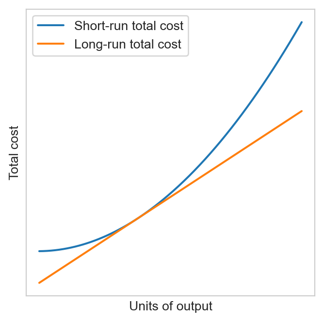
- Consider a firm with Cobb-Douglas production \(f = L^a K^b\) where \(K=\bar{K}>0\) is fixed in the SR. Thus the cost function found above is the LR cost. The SR cost can be found by solving the CMP with respect to \(L\) only
7.4.4 Average and marginal costs
Total cost of production: fixed costs + variable costs
Average cost (AC): total cost of production per output unit:
\[ AC(q) = \frac{C(q)}{q}, \tag{14}\] where \(C(q)\) is the total cost.
Marginal cost (MC): the rate at which the total cost increases as the firm produces an additional unit of output. Graphically it is the slope of the total cost curve:
\[ MC(q) = C'(q) \tag{15}\] in the continuous case.1
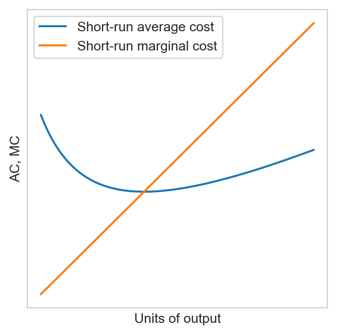
The MC curve crosses the AC curve at the AC’s minimum (if it has a minimum). In other words, the AC is decreasing when it is above the MC and increasing when it is above the MC.
Intuition:
- Initially when output is small, the variable cost is small and the fixed cost dominates the total cost. The extra cost of producing an additional unit is small, so the MC is below the AC and the AC is decreasing.
- As output increases, the importance of fixed cost declines. Meanwhile, the MC increases (due to decreasing marginal product)
- After a threshold, producing an additional unit costs more than the AC of existing units
8 Exercises
Exercise 2 For each of the following production functions, set up and solve the CMP.
- Cobb-Douglas production function: \(f(L,K) = L^a K^b\) where \(a, b>0\) and \(a+b=1\)
- Linear production function: \(f(L,K) = aL + bK\) where \(a, b>0\)
- Hint: Consider 3 cases: \(w/r = a/b\), \(w/r < a/b\) and \(w/r > a/b\)
Exercise 3 Consider again the Cobb-Douglas production function in Exercise 2. Let \(K(w, r, m)\) and \(L(w, r, m)\) denote the input demand for capital and labor, respectively.
- How do input demands change with the ouput level \(m\), and the input price?
- Are they homogeneous functions? If yes of which degree?
Exercise 4 Derive the cost function for a firm with a Cobb-Douglas production function. Is it a homogenous function? Of which degree? Explain.
Exercise 5 Let \(f = L^{1/2} K^{1/2}\) be the production function. Suppose that in the short run capital is fixed at \(\bar{K}=150\). Find the long-run and short-run cost functions. Which one is smaller? Does it make sense?
Exercise 6 Suppose \(w=\$40\) and \(r=\$10\). Derive the average and the marginal costs for the Cobb-Douglas production function \(f = L^{1/2} K^{1/2}\) in the SR and the LR.
Footnotes
It is equal to \(\Delta C / \Delta q\) in the discrete case↩︎