Chapter 1. Consumers and demand

1 Consumer preferences

1.1 Bundles

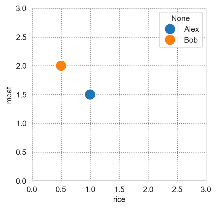
In economics, a bundle is a list or a vector of quantities of goods and services. In an \(n\)-good economy, each bundle \(x\) is an element of \(\mathbb{R}^n\). In the example below, the consumption bundle of Alex is \(x_A = (1, 1.5)\). If we know the prices of these goods in the economy, we can calculate the cost of his consumption as the dot product of the price vector and the consumption bundle. In addition, if we know his income, we can express his budget constraint mathematically as: \(p\cdot x_A \leq I_A\), where \(p\) is the price vector and \(I_A\) is Alex’s income.

Figure 1: Consumption bundle with two goods

1.2 The preference relation

Learning about preferences for bundles is essentially learning about how individuals compare bundles. Let us have a look at some key properties of the preference relation, namely: reflexivity, completeness, transitivity, continuity, monotonicity and (local) nonsasiation.

1.2.1 Notations

Before discussing these properties, let us fix the notations. Let \(x\) and \(y\) be two consumption bundles (or alternatives) in the set \(X \subset \mathbb{R}^n\) (the set of alternatives or the choice set). Then for some individual \(i\):

Preference	Notation
\(i\) weakly prefers \(x\) over \(y\)	\(x \succeq_i y\)
\(i\) strictly prefers \(x\) over \(y\)	\(x \succ_i y\)
\(i\) is indifferent between \(x\) and \(y\)	\(x \sim_i y\)

When it is clear from context that we will eliminate the letter \(i\) from the notations. Note that the equivalence relation \(\sim\) simply means that \(x\succeq y\) and \(y\succeq x\) . We also refer to the preference relation \(\succeq\) as the weak preference relation, as opposed to the strict preference relation \(\succ\).

To facilitate comparison, we shall also fix the following notations:

Notation	Meaning
\(x \geq y\)	\(x_j \geq y_j\) for all good \(j=1,2, \dots, n\).
\(x \gt y\)	\(x_j > y_j\) for all good \(j=1,2, \cdots, n\).

For example we typically assume that goods’ prices are strictly positive \(p\gt 0\), which we sometimes write \(p \in \mathbb{R}^n_{++}\). The notation \(x\ge y\) means that the quantity of each good in \(x\) is at least as much as that in \(y\), whereas \(x\gt y\) means that \(x\) has strictly more of every good than \(y\). The former permits \(x=y\) but the latter does not.

1.2.2 Reflexivity

A preference relation satisfies reflexivity if it any alternative is weakly preferred to itself, i.e., \(x \succeq x\) for any \(x\in X\).

1.2.3 Completeness

A preference relation over the set of alternatives \(X\) is complete if for any \(x\) and \(y\) in \(X\), either \(x \succeq y\), \(y \succeq x\), or both (\(x \sim y\)). Observe that a strict preference of \(y\) over \(x\) would be equivalent to \(x \succeq y\) and \(y \not\succeq x\).

Intuitively completeness conveys the property that one can rank any two alternatives; it is not possible to answer “I don’t know” when ask to make a comparison between two bundles.

1.2.4 Transitivity

Let \(A\), \(B\) and \(C\) be three alternatives. A preference relation is said to be transitive if:

\[ A \succeq B \text{ and } B \succeq C \implies A \succeq C. \tag{1}\]

Preferences that are both complete and transitive are said to be rational.

Condition Equation 1 might seem obvious at first sight, but evidence of intransitivity is rather prevalent. One of the most remarkable reasons for intransitivity is framing, the idea that ranking of preferences depends on the context. For example, one might prefer a mango to an avocado when thinking of them as fruits, but might prefer an avocado to a mango when thinking of making a salad. Other causes of intransitivity include cognitive difficulty when comparing close alternatives, or when each alternative involves multiple criteria (see textbook for details).

1.2.5 Monotonicity

Consider two alternatives \(A\) and \(B\) in \(X\subset \mathbb{R}^n\). We say that the preference relation \(\succeq\) satisfies monotonicity if the following conditions are satisfied:

\[ \begin{aligned} A \geq B \text{ and } a_k \neq b_k \text{ for some } k &\implies A \succeq B, \\ A \gt B &\implies A \succ B. \end{aligned} \tag{2}\]

A preference relation is said to satisfy strict monotonicity if:

\[ A \geq B \text{ and } a_k \neq b_k \text{ for some } k \implies A \succ B. \tag{3}\]

Strict monotonicity implies that we cannot have bads in the bundle. Monotonicity implies that we cannot have all bads in the bundle, otherwise \(A>B\) would imply the contrary. Note that a bad, as opposed to a good, is something we dislike (for e.g., trash); we pay to acquire a good, but to get rid of a bad.

1.2.6 Nonsatiation and local nonsatiation

1.2.6.1 Nonsatiation

A preference relation satisfies nonsatiation (NS) if for every bundle, there exists a strictly preferred bundle. Let \(X\) be the set of all alternatives or bundles, then NS implies that for any \(A\in X\) there exists \(B\in X\) such that:

\[ B \succ A \]

Remark 1.

• NS allows some of the items in the bundle to be bads
• NS implies that the consumer can always find something strictly better (no best bundle)

1.2.6.2 Local nonsatiation

On the other hand, a preference relation satisfies local nonsatiation (LNS) if for every bundle there exists in strictly preferred bundle within any \(\epsilon\)-distance from it (i.e. \(B \in N_{\epsilon} A\) for all \(\epsilon > 0\)). Mathematically,

\[ \forall A \in X,\: \forall \epsilon > 0: \: \exists B \in N_{\epsilon} A \text{ s.t. } B \succ A. \tag{4}\]

Remark 2.

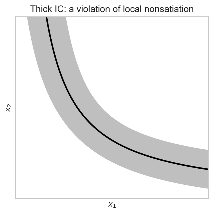
• LNS rules out thick indifference curves
• LNS is stricter than NS; in the former a better bundle must be found in any arbitrarily close alternative whereas in the latter it could be any other bundle in the choice set.

1.2.7 Relationships between properties

Here is a quick summary of the relationships between monotonicity, SM, NS, LNS:

\[ \begin{aligned} \text{S.Monotonicity } &\Rightarrow \text{ Monotonicity } \Rightarrow \text{ LNS} \Rightarrow \text{ NS} \\ \text{NS } &\nRightarrow \text{LNS } \nRightarrow \text{ Monotonicity} \nRightarrow \text{ S.Monotonicity} \end{aligned} \]

1.2.8 Continuity

Continuity (together with rationality) is needed to guarantee a utility representation of a preference relation.

• A preference relation defined on the set of alternatives \(X\) is continuous if it is preserved under limits.

  • For any sequence \(\{(x^n, y^n)\}_{n=1}^{\infty}\) with \(x^n \succeq y^n\) for all \(n\) and \(\lim_{n\to\infty} x^n = x\) and \(\lim_{n\to\infty} y^n = y\), it holds \(x \succeq y\).

• Intuitively, continuous preferences mean that there can be no sudden jumps (preference reversals) in an individual preference over a sequence of bundles

• Example of violation of continuity: lexicographic preferences (See exercise)

1.3 Utility functions

Utility was first used in the context of economics by Jeremy Bentham (1748-1832) as a measure of pleasure, happiness or satisfaction derived from the consumption of goods and services.

The utility function was first introduced by the Swiss mathematician Daniel Bernoulli (1700-1782) in the context of probability (gambling) to account for the St. Petersburg paradox

Theorem 1 (Existence) If a preference relation \(\succeq\) is rational (complete and transitive) and continuous on the set of alternatives \(X\subset \mathbb{R}^n\), then it can be represented by a continuous utility function \(u: X \to \mathbb{R}.\)

A utility function \(u: X \to \mathbb{R}\) is said to represent a preference relation \(\succeq\) over \(X\) if for all \(A, B \in X\), it holds \(A \succeq B \iff u(A) \geq u(B)\). In other words, ranking bundles is equivalent to ranking utilities assigned to them.

Very important: A utility function is not unique. If \(u\) represents \(\succeq\), then for any strictly increasing function \(f\), the function \(f \circ u\) also represents \(\succeq\). This is because if \(u(A) \geq u(B)\), then \(f(u(A)) \geq f(u(B))\) since \(f\) is strictly increasing.

Let us now look at some common properties of a utility function. Ideally, these properties should correspond to those desired of a preference relation.

1.3.1 Ordinality

• Utilities are ordinal (not cardinal)
  • \(u(A) = 2 u(B)\) means that \(A\) is strictly preferred but NOT twice as preferred as \(B\)
  • Example: IMDb Movies ratings on a scale from 1 to 10. A movie rated 8-star is better than one rated 4-star, but this doesn’t mean that the former is twice greater (maybe slightly, maybe infinitely so, we just don’t know from looking at utilities)
• This implies that any positive monotonic transformation of a utility function also represents the same preference relation as as that utility function.
  • In particular, if \(u\) represents \(\succeq\) then for any strictly increasing function \(f\), the function \(f \circ u\) also represents \(\succeq\).

1.3.2 Monotonicity

Let \(x\) and \(y\) be two alternatives in \(X \subset \mathbb{R}^n\). Then:

• Monotonic preferences \(\iff\) (weakly) increasing utility functions
  • Preferences: \(x \geq y \implies x \succeq y\) and \(x \gt y \implies x \succ y\)
  • Utility: \(x \geq y \implies u(x) \geq u(y)\) and \(x \gt y \implies u(x) > u(y)\)
• Strictly monotonic preferences \(\iff\) strictly increasing utility functions
  • Preferences: \(x \geq y \text{ and } x \neq y \implies x \succ y\)
  • Utility: \(x \geq y \text{ and } x \neq y \implies u(x) > u(y)\)

Example 1 (Perfect complements) The utility function \(u: X\subset\mathbb{R^2}\to\mathbb{R}\) defined by \(u(x_1, x_2)=\mathrm{min}\{ax_1, bx_2\}\) where \(a>0\) and \(b>0\) represents a monotonic but not strictly monotonic preference relation.

Example 2 (Perfect substitutes) The utility function \(u: X\subset\mathbb{R^2}\to\mathbb{R}\) defined by \(u(x_1, x_2)=ax_1 + bx_2\) where \(a>0\) and \(b>0\) represents a strictly monotonic preference relation.

Since monotonicity implies LNS (which in turns implies NS), both of these utility functions satisfy LNS and NS.

1.4 Indifference set

Figure 2: Indifference set, upper and lower contour sets

1.4.1 Implication of LNS

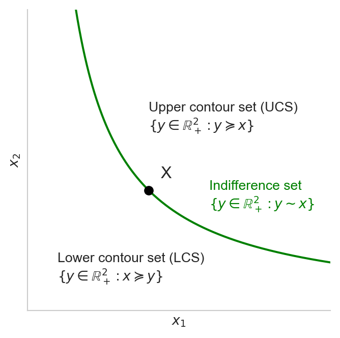
We have stated above that LNS implies that the ICs cannot be thick since if it were the case we would be able to find a sufficiently small neighborhood in which no alternative is strictly better than any other.

Figure 3: LNS rules out thick IC (in gray)

1.4.2 Implication of strict monotonicity

Why do we often see that the ICs are downward sloping? It is because of strict monotonicity. Indeed, let \(u(x, y)\) be a utility function representing strictly monotonic preferences. For simplicity suppose that \(u\) is differentiable, then the partial derivatives of \(u(\cdot)\) with respect to each argument, \(u_x\) and \(u_y\), are strictly positive. Along an IC, the level of utility is constant. By totally differentiating, we get:

\[ \begin{aligned} u_x dx + u_y dy &= 0 \\ \frac{dy}{dx} &= -\frac{u_x}{u_y}\\ &<0. \end{aligned} \tag{5}\]

1.4.3 Convexity of preferences

Convexity of preferences captures an individual’s taste for diversification. Formally, we say that preferences are convex if the upper-contour set (UCS) is a convex set.¹

Figure 4: Convex UCS (shaded) and preferences for diversification. Observe that any mix of \(x\) and \(y\) is strictly preferred to \(z\).

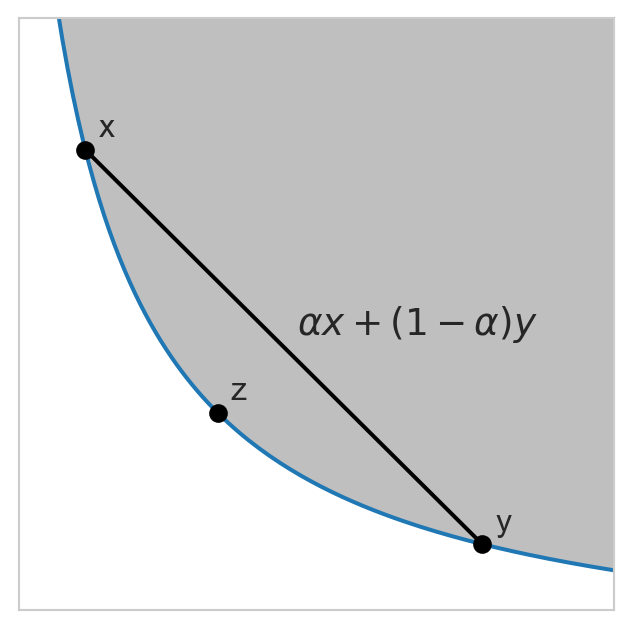
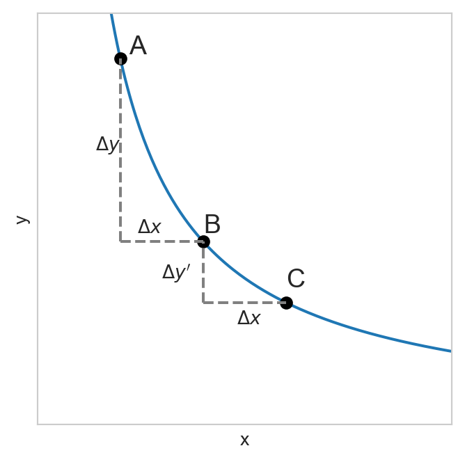
Convexity implies diminishing marginal rates of substitution, the term on the RHS of Equation 5 (in absolute value):

\[ MRS_{y, x} \equiv \frac{u_x}{u_y} = -\frac{dy}{dx}. \tag{6}\]

The MRS captures our willingness to exchange one good for an additional unit of another. In particular, \(MRS_{y,x}\) captures the amount of good \(y\) the individual is willing to give up for an additional unit of good \(x\) in order to maintain the same level of utility. The intuition behind a decreasing MRS is that as one good gets abundant, we are willing to sacrifice less of the other good for an additional unit of the abundant good. This is due to the preference for variety captured by convexity.

Figure 5: Diminishing marginal rates of substitution

1.4.4 Concavity and quasiconcavity

Definition 1 (Quasiconcavity 1) A utility function defined on a convex set \(X\) is quasiconcave if for all \(x \in X\), the upper contour set of \(x\), defined by \(\mathrm{UCS}(x) = \{y \in X: u(y) \geq u(x)\}\), is convex.

An alternative definition of quasiconcavity is the following.

Definition 2 (Quasiconcavity 2) A utility function \(u\) defined on a convex set \(X\) is quasiconcave if for all \(x, y \in X\): \[ u(\alpha x + (1 - \alpha) y) \geq \min\{u(x), u(y)\}. \] It is strictly quasiconcave if: \[ u(\alpha x + (1 - \alpha) y) > \min\{u(x), u(y)\}. \]

Concavity implies quasiconcavity (proof as exercise). Quasiconcavity is preserved under a strictly increasing transformation, which makes it a desirable property of utility functions since representation is not unique. To check quasiconcavity, it is often easier to check the quasiconcavity of its transformation. If a strictly increasing transformation of a utility function is concave, then the orginal utility function is quasiconcave (not necessarily concave), why?

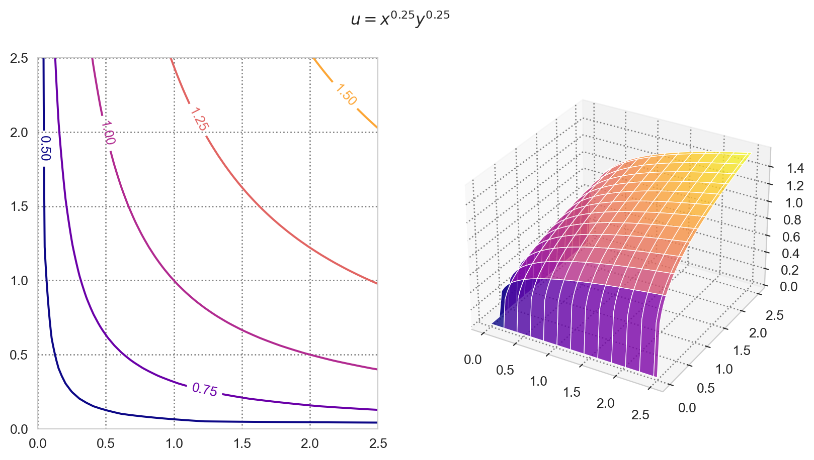
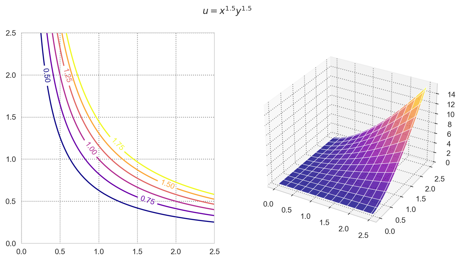
Quasiconcavity does not imply concavity. For example, consider the Cobb-Douglas utility function \(u=x^a y^b\), where \(a,b>0\). Suppose \(a=b=1/4\), then \(u\) is strictly concave, hence is also quasiconcave. For \(a=b=3/2\), the utility function is quasiconcave but not concave.

Concave utility function and indifference curves

Quasiconcave utility function and indifference curves

1.5 Homogeneity and homotheticity

1.5.1 Homogeneity

Definition 3 (Homogeneous function) A function \(u:\mathbb{R}^n\to\mathbb{R}\) is homogeneous of degree \(k\) if for all \(\alpha > 0\), we have \(u(\alpha x) = \alpha^k u(x)\).

• Varying the amount of goods by a common factor \(\alpha\) changes the utility by a factor \(\alpha^k\).
  • \(\alpha > 1\): an increase
  • \(\alpha \in (0, 1)\): a reduction
• For a production function, the degree of homogeneity tells us about returns to scales of the production technology. In particular:
  • \(k<1\): DRS
  • \(k=1\): CRS
  • \(k>1\): IRS

Definition 4 (Homogeneous preference) A preference relation is homogeneous if it can be represented by a homogeneous utility function

1.5.1.1 Properties

1. If \(u\) is homogeneous of degree \(k\), then its first-order partial derivatives are homogeneous of degree \(k-1\): \[ u(\alpha x) = \alpha^k u(x) \implies u_j(\alpha x) = \alpha^{k-1} u_j(x). \tag{7}\]

2. The ICs of homogeneous functions are radial expansions of one another, i.e., if \(x\) and \(y\) lie on the same IC, then so are \(\alpha y\) and \(\alpha x\): \[ u(x) = u(y) \implies u(\alpha x) = u(\alpha y). \tag{8}\]

   • Knowing the shape of a single IC tells us the shape of all other ICs

3. The MRS of a homogeneous function is constant for all points along each ray from the origin (homogeneity of degree \(0\)): \[MRS_{1,2}(x) = MRS_{1,2}(\alpha x), \quad \forall x\in X.\]

Proof

Proof.

1. Partially differentiating w.r.t \(x_i\) yields: \[ \begin{aligned} \frac{\partial u(\alpha x)}{\partial (\alpha x_j)}\alpha &= \alpha^k \frac{\partial u(x)}{\partial x_j} \\ u_j(\alpha x) &= \alpha^{k-1} u_j(x). \end{aligned} \]

2. This comes from the definition: \[ u(x) = u(y) \iff \alpha^k u(x) = \alpha^k u(y) \iff u(\alpha x) = u(\alpha y). \]

3. This can be proven by using the first property: \[ \begin{aligned} MRS_{1,2}(x) \equiv \frac{U_1(x)}{U_2(x)} &= \frac{\alpha^{k-1}U_1(x)}{\alpha^{k-1}U_2(x)} \\ &= \frac{U_1(\alpha x)}{U_2(\alpha x)}. \end{aligned} \]

1.5.2 Homotheticity

Definition 5 (Homothetic function) A function \(u:\mathbb{R}^n\to\mathbb{R}\) is homothetic if it is obtained by a monotonic transformation of a homogeneous function (Definition 3), i.e., if there exist a strictly increasing function \(f:\mathbb{R}\to\mathbb{R}\) and a homogeneous function \(v:X\to\mathbb{R}\) such that:

\[ u(x) = f(v(x)). \tag{9}\]

Clearly, a homogeneneous function is also homothetic (let \(f\) be the identity function). Importantly, homotheticity is preserved under a monotone transformation whereas homogeneity is not. It is thus a desirable property of utility functions. As in the case of homogeneity, we can also talk about homothetic preferences.

Definition 6 (Homothetic preference) A preference relation is homothetic if it can be represented by a homothetic utility function (Definition 5).

Since a homogeneous utility function is homothetic, homogeneous preferences are also homothetic, but the converse is not true.

1.5.2.1 Properties

1. ICs are radial expansion of the origin: \(x \sim y \implies \alpha x \sim \alpha y\) for all scalar \(\alpha > 0\)

2. MRS is homogeneous of degree \(0\): The rate at which the individual substitutes one good for another depends only on the proportion of the two goods consumed, and not on:

   • the utility level obtained
   • the absolute quantities of the goods

3. Homotheticity is preserved under a monotonic transformation, while homogeneity is not

Proof

• Suppose \(u\) is homothetic. We want to show \(u=f(v(x))\) for some homothetic \(v\) and strictly increasing function \(f\). Since \(v\) is homothetic there exists a strictly increasing function \(h\) and a homogeneous function \(t\) such that \(v=h(t(x))\). Hence \(u=f(h(t(x))) = (f\circ h) (t(x))\) where \(f\circ h\) is strictly increasing. This shows that \(u\) is a monotonic transformation of \(t\), a homog function, hence is homothetic

• That homogeneity is not preseved under a monotonic transformation can be shown by a counter example. For instance, consider \(u(x, y) = xy\), which is homogeneous of degree 2 (why?), but the monotone transformation \(f(u) = u + a\) for some constant \(a>0\) is not.

1.5.3 Examples

• Constant elasticity of substitution (CES) utility function: \[ u(x, y) = [\alpha x^p + (1 - \alpha)y^p]^{1/p}, \tag{10}\] where \(p\neq 0\) and \(\alpha \in (0, 1)\).

  The CES function is a generalization of several other functions.

  • When \(p\) approaches 0, it becomes the Cobb-Douglas utility function
  • When \(p\) approachs \(-\infty\), we obtain \(u(x, y) = \min \{ax, by\}\), the Leontief utility function
  • When \(p=1\), we obtain \(u(x, y)= ax + by\), which represents preferences for perfect substitutes

• Constant relative risk aversion (CRRA) utility: \[ u(x) = \begin{cases} \frac{x^{1-\sigma}}{1-\sigma}, & \sigma>0,\: \sigma\neq 1 \\ \ln (x), & \sigma = 1. \end{cases} \] The CRRA utility function is used extensively in models of decision making under uncertainty.

2 Utility maximization and demand for goods and services

2.1 Utility maximization problem (UMP)

• Denote \(w>0\) the consumer’s wage/income, \(p\) the vector of prices, \(x\) the bundle of goods and services, and \(u:\mathbb{R}^L_+\to \mathbb{R}\) the utility function representing the preferences of the consumer. Futhermore, denote \(pw\) the dot product of \(p\) and \(w\) when they are vectors

• The UMP faced by the consumer is: \[ \max u(x) \text{ s.t. } px \leq w \tag{11}\]

• The budget set or budget constraint: \(B(p,w) \equiv \{x \geq 0: px \leq w\}\).

• If \(w>0\) and \(p > 0\) and \(u\) is continuous then a solution to the UMP exists (Weirestrass theorem)

• A solution to the UMP, if exists, is a list of goods and services that maximizes the utility of the consumer given her budget constraint.

2.2 Walrasian demand

• Let \(x(p,w)\) be the solution to the UMP: it is called the Walrasian demand correspondence

• For each \((p,w)\) pair, the correspondence specifies a set of optimal bundles

• If preferences are strictly convex, this set is a singleton: the correspondence becomes a function (Walrasian demand function)

2.2.1 Properties of the Walrasian demand correspondence

If the utility function is continuous and preferences satisfy LNS (thin ICs) over the consumption set \(\mathbb{R}^L_+\), then the Walrasian demand satisfies:

1. Homogeneity of degree \(0\): \(x(p,w) = x(\alpha p, \alpha w)\) for all \(p\gg 0\) and \(w>0\)
   • No monetary illusion: raising income by the same proportion as prices does not modify optimal consumption
   • Example: we receive a 10% raise but the cost of living also increases by 10%
   • Formally, this is because the budget set is unchanged; the UMP being the same, so is its solution
2. Law of Walras (LoW): \(px = w\) for all \(x=x(p,w)\)
   • This follows from LNS: Any bundle in the interior of the budget set is not optimal since there exists another bundle strictly better in a sufficiently small neighborhood of this bundle
3. Convexity: If preferences are convex, then \(x(p,w)\) defines a convex set. If moreover preferences are strictly convex, then \(x(p,w)\) contains a singleton

2.3 Solving the UMP

2.3.1 Necessary conditions

The Lagragian associated with the UMP:

\[ L = u(x) + \lambda (w - px) \tag{12}\]

Denote \(L_i\) the partial derivative of the Lagrangian with respect to good \(i\). The KTT theorem tells us that if \(x^*\) is a solution to the UMP then there exists \(\lambda^*\geq 0\) such that the following conditions are satisfied: \[ \begin{aligned} & L_i(x^*) \equiv \frac{\partial L}{\partial x_i}(x^*) = 0, \quad i=1,\dots, L \\ % & L_i(x^*) = 0 \text{ if } x^*_i>0, \quad i=1,\dots,L \\ & \lambda^* \geq 0, \: w - px^* \geq 0 \text{ and } \lambda^*(w - px^*) = 0. \end{aligned} \tag{13}\]

The first set of conditions yields \[ u_i(x^*) = \lambda^* p_i. \]

If \(u\) satisfies strict monotonicity (\(u_i>0\)), then \(\lambda^*>0\) since prices are strictly positive. But \(\lambda^*>0\) implies that \(w = px^*\), which confirms the LoW.

To eliminate the multiplier, we can form the ratio: \[ \begin{aligned} \frac{u_i(x^*)}{u_j(x^*)} &= \frac{p_i}{p_j} \\ MRS_{j,i}(x^*) &= \frac{p_i}{p_j} \\ \implies \frac{u_i(x^*)}{p_i} &= \frac{u_j(x^*)}{p_j} = \lambda^*. \end{aligned} \tag{14}\]

Hence at an optimum:

• The rate at which the individual substitutes one good for the other is equal to the ratio of their prices - the market value of one good relative to the other good. Price levels do not matter

• Marginal utilities per unit of the constraint (e.g. dollar) are equalized across all goods and are equal to the Langrage multiplier, the shadow price

2.3.2 The shadow price

• \(\lambda^*\) is often interpreted as the shadow price: the increase in the maximized objective function (indirect utility in this context) as the constraint is relaxed by one unit

• In other words, it is the shadow price on the constraint (on \(w\))

• Mathematically: \[ \lambda^* = \frac{\partial u(x^*(p,w))}{\partial w} \equiv \frac{\partial v}{\partial w}, \]

where \(v(p,w) = u(x^*(p,w))\) is called the indirect utility function.

Proof

We can show this by differentiating the value function w.r.t income: \[ \begin{aligned} \frac{\partial u(x^*(p,w))}{\partial w} &= \sum_{i=1}^L u_i(x^*)\frac{\partial x_i(w,p)}{\partial w} \\ &= \lambda^*\sum_{i=1}^L p_i \frac{\partial x_i(w,p)}{\partial w} \\ &= \lambda^*. \end{aligned} \]

The second line comes from the first-order conditions Equation 14. And the third line comes from the fact the budget constraint binds at the optimum, which implies: \[ \sum_{i=1}^L p_i \frac{\partial x_i(w,p)}{\partial w} = 1. \]

2.3.3 Sufficient conditions

• How to be sure that the necessary conditions above provide a max, and not a min?

• The KKT conditions are also sufficient for a max if:

  1. \(u\) is quasiconcave
     • UCS is convex
  2. \(u\) is monotone
     • ICs are downward sloping
  3. \(u_i(x) \neq 0 \: \forall i \iff \nabla u(x) \neq 0\)
     • There is no bliss point
     • If such a point existed then LNS would be violated, which would contradict monotonicity

2.3.4 Example: Cobb-Douglas utility function with availability constraints

Let us consider the Cobb-Douglas utility function \(u(x_1, x_2) = x_1^{\alpha}x_2^{1-\alpha}\) with \(\alpha\in(0,1)\). The consumer faces the budget constraint \(p_1x_1 + p_2x_2 \leq w\) (Case 1) and an availability constraint on one of the goods \(x_1 \leq \bar{x}_1\) or \(x_2 \leq \bar{x}_2\) (Case 2). Play around with the interactive below to see how the optimal bundle changes as we vary the parameters of the problem.

2.4 Comparative statics

1. Price elasticity: percentage change in demand following a percentage change in the price of the good:

   \[ \epsilon_{x_i, p_i} = \frac{\partial x_i(p,w)}{\partial p_i}\frac{p_i}{x_i(p,w)}. \tag{15}\]

   • If positive: Giffen goods
   • If negative: normal goods

2. Cross-price elasticity: percentage change in the demand of a good following a percentage change in the price of another good:

   \[ \epsilon_{x_i, p_j} = \frac{\partial x_i(p,w)}{\partial p_j}\frac{p_j}{x_i(p,w)}. \tag{16}\]

   • If positive: substitutes
   • If negative: complements

3. Income elasticity: percentage change in the demand of a good following a percentage change in income:

   \[ \epsilon_{x_i, w} = \frac{\partial x_i(p,w)}{\partial w}\frac{w}{x_i(p,w)}. \tag{17}\]

   • If postive: normal goods
   • If negative: inferior goods

---

3 Exercises

Exercise 1 (Lexicographic preferences) Consider the preference relation over \(X=\mathbb{R}^2_+\) as follows: \[ \forall x, y \in X:\: x \succeq y \text{ if } \begin{cases} x_1 > y_1, \text{ or} \\ x_1 = y_1 \text{ and } x_2 > x_1 \end{cases} \]

It is called lexicographic because it resembles the way we look up a word in a paper dictionary. Why does such a preference violate continuity?

Answer

Consider the sequence \(x^n=(1/n, 0)\) and \(y^n=(0, 1)\), for \(n=1,2,...\) Observe that \(x^n \succeq y^n\) for all finite \(n\), but \(\lim y^n = (0,1) \succeq \lim x^n = (0,0)\).

Exercise 2 (St. Petersburg paradox) St.Petersburg paradox: We pay a fee to play a game of chance in which we toss a fair coin until the first it turns heads. The prize is \(2^k\) where \(k\) is the round on which the first head is obtained. Most people are not willing to pay more than a few dollars to play the game, does it make sense? What is the expected value (EV) of the game?

Answer

The expected value of this game is \(\sum_k (1/2)^k 2^k = 1 + 1 + ... = \infty.\) One way to explain this paradoxical behavior is to model preferences using a bounded utility function. The individual is then willing to pay up to the certainty equivalent of the game given her utility function. For a concave utility function, which captures risk aversion, the certainty equivalent is smaller than the expected value of the game. In particular, it can be shown that if the utility function is logarithmic, the certainty equivalent is 4.

Exercise 3 (Convex preferences) Please verify the convexity and strict convexity of preferences represented by the utility functions in the following table.

\[ \begin{array}{l|c|c} \hline u(x_1, x_2) & \text{Convex} & \text{Strictly convex} \\ \hline ax_1 + bx_2 & \checkmark & \times \\ \min\{ax_1, bx_2\} & \checkmark & \times \\ ax_1^2 x_2^2 & \checkmark & \checkmark \\ ax_1^{\frac{1}{2}} + bx_2^{\frac{1}{2}} & \checkmark & \checkmark \\ ax_1^2 + bx_2^2 & \times & \times \\ \hline \end{array} \]

Exercise 4 (Monotonicity) Prove that the utility function in Example 1 satisfy monotonicity but not strict monotonicity, and the utility function in Example 2 satisfy monotonicity.

Exercise 5 Prove that (strict) concavity implies (strict) quasiconcavity.

Answer

• A function \(u:X\to \mathbb{R}\) is concave if for all \(x, y \in X\) and \(\alpha \in (0,1)\):

  \[ u(\alpha x + (1 - \alpha) y) \geq \alpha u(x) + (1-\alpha) u(y) \tag{18}\]

• Since \(u(x) \geq \min\{u(x), u(y)\}\) and \(u(y) \geq \min\{u(x), u(y)\}\):

  \[ \begin{aligned} u(\alpha x + (1 - \alpha) y) &\geq \alpha u(x) + (1-\alpha) u(y) \\ &\geq \alpha \min\{u(x), u(y)\} + (1-\alpha)\min\{ u(x), u(y)\} \\ &= \min\{u(x), u(y)\} \end{aligned} \tag{19}\]

• That strict concavity implies strict quasiconcavity can be proven in the same fashion

Exercise 6 Consider the Cobb-Douglas utility function \(u(x,y)=x^{1/3}y^{2/3}.\) Is it concave? quasiconcave? homogeneous? homothetic? How about its log transformation?

Exercise 7 (Walrasian demand) Consider the Cobb-Douglas utility function over two goods defined by \(u(x,y)=x^a y^b\), where \(a,b>0\) and \(a+b=1\). Let \(p > 0\) the price vector and \(w>0\) the income of the individual.

1. Write the UMP faced by the individual

2. Form the Lagragian

3. What are the KKT necessary conditions? Are they also sufficient? What is the meaning of the Lagrange multiplier?

4. Find the Walrasian demand

5. Verify that the Walrasian demand you have found satisfies the three properties above, namely homogeneity of degree \(0\), LoW and convexity

6. Compute the common elasticities presented in the lecture and comment

Footnotes

1. A convex set is a set that contains all its convex combinations. Let \(x\) and \(y\) be any two points in a set \(A\), then \(A\) is called a convex set if for any \(\alpha \in [0, 1]\), any convex combination of \(x\) and \(y\), \(\alpha x + (1-\alpha)y\) also belongs to A. Graphically, if we fix any two points in a convex set and draw a line between them, the line is contained in the set.